Alpha diversity
Contents
9. Alpha diversity
In this chapter we’ll begin to explore metrics of microbiome diversity. We’ll start with metrics of alpha diversity, which are measures of “within-sample” diversity. The way I typically think of these is as metrics that can be computed on a single sample.
The first sub-category of alpha diversity metric that we’ll look at will be richness. Richness refers to how many different types of organisms are present in a sample. For example, if we’re interested in species richness of plants in the Sonoran Desert and the Costa Rican rainforest, we could go to each, count the number of different species of plants that we observe, and have a basic measure of species richness in each environment.
Jargon: “type of organism”
As defined earlier, a “type of organism” or a “type of microbe” is an arbitrary taxonomic grouping, such as genus, species, strain, or even an amplicon sequence variant.
The next sub-category of alpha diversity metric that we’ll discuss in this chapter will be evenness. Evenness tells us how consistent the distribution of species abundances are in a given environment. If, for example, the most abundant plant in the Sonoran desert was roughly as common as the least abundant plant (not the case!), we would say that the evenness of plant species was high. On the other hand, if the most abundant plant was thousands of times more common than the least common plant (probably closer to the truth), then we’d say that the evenness of plant species was low.
9.1. Metrics of microbiome richness
We’ll begin by looking at two metrics of community richness. Both of these are commonly used in practice.
9.1.1. Observed features
Observed features is a very simple metric that can be used to quantify microbiome diversity. With this metric, we simply count the features that are observed in a given sample. A feature is considered to have been observed in a sample if it has a frequency of greater than zero. This is a qualitative diversity metric meaning that each feature is treated as being either observed or not observed. This metric doesn’t consider how many times a feature was observed.
Let’s define a simple feature table for this analysis:
import pandas as pd
import numpy as np

sample_ids = ['4ac2', 'e375', '4gd8']
feature_ids = ['B1','B2','B3','B4','B5','A1','E2']
data = np.array([[5, 5, 2, 0, 0, 0, 0],
                 [3, 5, 1, 4, 4, 0, 0],
                 [5, 0, 0, 0, 0, 5, 5]])

feature_table_1 = pd.DataFrame(data, index=sample_ids, columns=feature_ids)
feature_table_1.style
| B1 | B2 | B3 | B4 | B5 | A1 | E2 | |
|---|---|---|---|---|---|---|---|
| 4ac2 | 5 | 5 | 2 | 0 | 0 | 0 | 0 |
| e375 | 3 | 5 | 1 | 4 | 4 | 0 | 0 |
| 4gd8 | 5 | 0 | 0 | 0 | 0 | 5 | 5 |
To compute the value of observed features for each sample in our feature table, we would simply count the number of non-zero counts for each sample. All of the non-zero counts are bolded in the following view of the table.
def non_zero_blue(frequency):
    if frequency > 0:
        color = 'blue'
    else:
        color = 'black'
    return 'color: %s' % color

feature_table_1.style.applymap(non_zero_blue)
| B1 | B2 | B3 | B4 | B5 | A1 | E2 | |
|---|---|---|---|---|---|---|---|
| 4ac2 | 5 | 5 | 2 | 0 | 0 | 0 | 0 |
| e375 | 3 | 5 | 1 | 4 | 4 | 0 | 0 |
| 4gd8 | 5 | 0 | 0 | 0 | 0 | 5 | 5 |
Counting non-zero values for each sample would result in the following values of observed features for each sample:
import qiime2
import qiime2.plugins.diversity as div

feature_table_1a = qiime2.Artifact.import_data("FeatureTable[Frequency]", feature_table_1)

observed_features_1a = div.actions.alpha(feature_table_1a, metric='observed_features').alpha_diversity
observed_features_1 = observed_features_1a.view(pd.Series).to_frame(name='observed-features')
observed_features_1.style
| observed-features | |
|---|---|
| 4ac2 | 3 |
| e375 | 5 |
| 4gd8 | 3 |
Based on the observed features metric, we could consider samples 4ac2 and 4gd8 to have equal feature richness, and sample e375 to have a higher feature richness. Also note that while 4ac2 and 4gd8 have the same feature richness, different features are present in the two samples. Richness tells us only about how many different features are present, but nothing about which features are present.
Simple counting of features, as we’re doing here, is common but there are a few limitations to be aware of.
9.1.2. Even sampling
Imagine again that we’re going on a sampling trip to count plants in the Sonoran Desert and the Costa Rican rainforest. We’re interested in getting an idea of the plant richness in each environment. In the Sonoran Desert, we survey a square kilometer area, and count 150 species of plants. In the rainforest, we survey a square meter, and count 15 species of plants. On the basis of our survey we decide that plant species richness is higher in the desert than in the rainforest. Where did we go wrong?
We expended a lot more sampling effort in the desert than we did in the rainforest, so it shouldn’t be surprising that we observed more species there. If we expended the same effort in the rainforest, we’d probably observe a lot more than 15 or 150 plant species, and we’d have a more sound comparison.
In sequencing-based studies of microbiomes, the analog of sampling area is sequencing depth. If we collect 100 sequences from one sample, and 10,000 sequences from another sample, we can’t directly compare the number of observed features across these samples because we expended a lot more sampling effort on the sample with 10,000 sequences than on the sample with 100 sequences.
The ideal way to normalize tables for computation of these metrics is a subject of ongoing research, and most likely differs depending on what you want to do with the feature table. We’ll cover this topic in Normalization of Feature Tables. At present, when computing alpha and beta diversity metics, the way this is typically handled is by randomly subsampling sequences without replacement at a fixed total frequency across all samples. This process is referred to as rarefaction. Continuing from the example above, if we randomly select 100 sequences to represent the sample with 10,000 sequences (i.e., we rarefy that sample to a depth of 100 sequences) we can compute its richness based on that random subsample. That richness value will serve as a more relevant comparison to the richness value for the sample that we only obtained 100 sequences from.
Warning
Rarefaction is not ideal. I think of it as a necessary evil that enables these comparisons. Our field needs to move toward better normalization techniques that are accessible to users to get beyond the need to rarefy data. You must rarefy or otherwise normalize your feature table data before computing alpha and beta diversity unless the metric you’re using specifically does not require this.
Because rarefaction involves taking a random subsample of sequences from each sample, rarefying the same feature table multiple times will yield different rarefied feature tables. This is sometimes managed by computing multiple rarefied feature tables, computing diversity metrics on each table, and then averaging the diversity value computed for each sample. We’ll explore this below in Alpha rarefaction.
The following are three different rarefied versions of our example feature table from above, each rarefied to 10 sequences per sample. Notice that the total frequency for each sample is now ten. After rarefied, Observed Features is computed and presented for each rarefied table.
9.1.2.1. A rarefied feature table at sampling_depth=10
import qiime2.plugins.feature_table as ft

rarefied_feature_table_1a = ft.actions.rarefy(table=feature_table_1a, sampling_depth=10).rarefied_table
rarefied_feature_table1 = rarefied_feature_table_1a.view(pd.DataFrame).astype(int)
rarefied_feature_table1.style
| B1 | B2 | B3 | B4 | B5 | A1 | E2 | |
|---|---|---|---|---|---|---|---|
| 4ac2 | 4 | 4 | 2 | 0 | 0 | 0 | 0 |
| e375 | 1 | 3 | 0 | 3 | 3 | 0 | 0 |
| 4gd8 | 4 | 0 | 0 | 0 | 0 | 3 | 3 |
rarefied_observed_features_1a = div.actions.alpha(rarefied_feature_table_1a, metric='observed_features').alpha_diversity
rarefied_observed_features_1 = rarefied_observed_features_1a.view(pd.Series).to_frame(name='observed-features')
rarefied_observed_features_1.style
| observed-features | |
|---|---|
| 4ac2 | 3 |
| e375 | 4 |
| 4gd8 | 3 |
9.1.2.2. Another rarefied feature table at sampling_depth=10
rarefied_feature_table_2a = ft.actions.rarefy(table=feature_table_1a, sampling_depth=10).rarefied_table
rarefied_feature_table2 = rarefied_feature_table_2a.view(pd.DataFrame).astype(int)
rarefied_feature_table2.style
| B1 | B2 | B3 | B4 | B5 | A1 | E2 | |
|---|---|---|---|---|---|---|---|
| 4ac2 | 4 | 4 | 2 | 0 | 0 | 0 | 0 |
| e375 | 2 | 3 | 0 | 2 | 3 | 0 | 0 |
| 4gd8 | 5 | 0 | 0 | 0 | 0 | 1 | 4 |
rarefied_observed_features_2a = div.actions.alpha(rarefied_feature_table_2a, metric='observed_features').alpha_diversity
rarefied_observed_features_2 = rarefied_observed_features_2a.view(pd.Series).to_frame(name='observed-features')
rarefied_observed_features_2.style
| observed-features | |
|---|---|
| 4ac2 | 3 |
| e375 | 4 |
| 4gd8 | 3 |
9.1.2.3. A third rarefied feature table at sampling_depth=10
rarefied_feature_table_3a = ft.actions.rarefy(table=feature_table_1a, sampling_depth=10).rarefied_table
rarefied_feature_table3 = rarefied_feature_table_3a.view(pd.DataFrame).astype(int)
rarefied_feature_table3.style
| B1 | B2 | B3 | B4 | B5 | A1 | E2 | |
|---|---|---|---|---|---|---|---|
| 4ac2 | 4 | 4 | 2 | 0 | 0 | 0 | 0 |
| e375 | 2 | 1 | 1 | 3 | 3 | 0 | 0 |
| 4gd8 | 2 | 0 | 0 | 0 | 0 | 3 | 5 |
rarefied_observed_features_3a = div.actions.alpha(rarefied_feature_table_3a, metric='observed_features').alpha_diversity
rarefied_observed_features_3 = rarefied_observed_features_3a.view(pd.Series).to_frame(name='observed-features')
rarefied_observed_features_3.style
| observed-features | |
|---|---|
| 4ac2 | 3 |
| e375 | 5 |
| 4gd8 | 3 |
9.1.2.4. A rarefied feature table at a higher sampling depth (sampling_depth=13)
If instead of choosing to rarefy at ten sequences per sample (which is lower than the total frequency of any of our samples) we rarefied at thirteen sequences per sample (which is higher than the total frequency of sample 4ac2), sample 4ac2 will be dropped from the resulting feature table.
rarefied_feature_table_4a = ft.actions.rarefy(table=feature_table_1a, sampling_depth=13).rarefied_table
rarefied_feature_table4 = rarefied_feature_table_4a.view(pd.DataFrame).astype(int)
rarefied_feature_table4.style
| B1 | B2 | B4 | B5 | A1 | E2 | |
|---|---|---|---|---|---|---|
| e375 | 3 | 4 | 3 | 3 | 0 | 0 |
| 4gd8 | 5 | 0 | 0 | 0 | 5 | 3 |
rarefied_observed_features_4a = div.actions.alpha(rarefied_feature_table_4a, metric='observed_features').alpha_diversity
rarefied_observed_features_4 = rarefied_observed_features_4a.view(pd.Series).to_frame(name='observed-features')
rarefied_observed_features_4.style
| observed-features | |
|---|---|
| e375 | 4 |
| 4gd8 | 3 |
9.1.2.5. A limitation of feature counting
Imagine that we have the same table, but some additional context about the features in the table. Specifically, imagine we’ve computed the following phylogenetic tree from our feature sequences. And, for the sake of illustration, imagine that we’ve also assigned taxonomy to each of the features and found that our samples contain representatives from the archaea, bacteria, and eukaryotes (their labels begin with A, B, and E, respectively, in this example).
from io import StringIO
from skbio.tree import TreeNode

tree_1n = StringIO('((B1:0.1,B2:0.05):0.1,((B3:0.05,B4:0.1):0.1,B5:0.2):0.1,'
                   '((A1:0.1,A2:0.05):0.3,'
                   '(E1:0.1,E2:0.1):0.7):0.25);')

tree_1 = TreeNode.read(tree_1n)
tree_1 = tree_1.root_at_midpoint()

tree_1a = qiime2.Artifact.import_data("Phylogeny[Rooted]", tree_1)
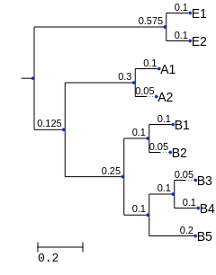
Fig. 9.1 A phylogenetic tree representing all of the features in our original feature table. (This tree isn’t intended to accurately represent the relationship between the Bacteria, Archaea, and Eukarya.)
Pairing this with the table we defined above (displayed again in the cell below), and given what you now know about these features, how do you feel about the relative richness of these samples?
9.1.3. Phylogenetic Diversity (PD)
Phylogenetic Diversity (PD or Faith’s PD) is a metric of richness that was developed in the early 1990s [Fai92]. Like many of the metrics that are used in microbiome research, it wasn’t initially designed for studying microbial communities, but rather communities of plants, animals, and other “macro-organisms” (macrobes?). Some of these metrics, including PD, do translate well to microbial community analysis, while others don’t.
PD is computed as the sum of the branch lengths in a phylogenetic tree that are represented in a given sample. I recommend computing this by hand on the example data presented in this chapter to ensure that you understand how it works. It can help to have a piece of scratch paper and to print out a copy of the phylogenetic tree (Fig. 9.1 in this example) to work through this process. It can also help to have a few colors of pencil or pen for this (one color per sample).
For each sample in a given feature table, write down which features ids were observed in that sample on a different line. Choose a color to use to represent this sample.
For each feature id in your list, find that feature in the phylogenetic tree. Trace from the feature id to the root node of the tree in the current sample’s color. As you trace, write down the branch lengths of any new branches that you trace in the current color for this feature. (If you encounter a branch that you have traced for a different feature in this sample, don’t write it down again.)
When you have done this for all of the features observed in the sample, sum the lengths of the branches that you wrote down. Again, each branch length should be added only one time for each sample. The resulting sum is the Phylogenetic Diversity of the sample.
Repeat this for each sample in the feature table. Remember to choose a new color for each sample.
Let’s apply this metric to the three rarefied feature tables that we computed above. For each rarefied feature table, I’ll print out what I would have written down on my scratch paper.
def phylogenetic_diversity(tree, table, sample_id, verbose=False):
    # Don't use this function in practice - it's untested and slow. Instead use
    # qiime2.plugins.diversity.actions.alpha_phylogenetic()

    if verbose:
        print("Observed branch lengths for sample %s" % sample_id)
    sample_vector = table.T[sample_id]
    observed_features = sample_vector.index[sample_vector.to_numpy().nonzero()[0]]
    observed_nodes = set()
    # iterate over the observed features
    for feature_id in observed_features:
        t = tree.find(feature_id)
        observed_nodes.add(t)
        if verbose:
            print(t.name, t.length, end=' ')
        for internal_node in t.ancestors():
            if internal_node.length is None:
                # we've hit the root
                if verbose:
                    print('')
            else:
                if verbose and internal_node not in observed_nodes:
                    print(internal_node.length, end=' ')
                observed_nodes.add(internal_node)
    result = sum([t.length for t in observed_nodes])
    if verbose:
        print()
    return result
9.1.3.1. Faith’s PD computed on our first rarefied feature table
The first rarefied feature table was as follows:
rarefied_feature_table1.style
| B1 | B2 | B3 | B4 | B5 | A1 | E2 | |
|---|---|---|---|---|---|---|---|
| 4ac2 | 4 | 4 | 2 | 0 | 0 | 0 | 0 |
| e375 | 1 | 3 | 0 | 3 | 3 | 0 | 0 |
| 4gd8 | 4 | 0 | 0 | 0 | 0 | 3 | 3 |
Working through the steps for each sample, I would have the following notes:
for sample_id in rarefied_feature_table1.index:
    _ = phylogenetic_diversity(tree_1, rarefied_feature_table1, sample_id, verbose=True)
Observed branch lengths for sample 4ac2
B1 0.1 0.1 0.25 0.125
B2 0.05
B3 0.05 0.1 0.1

Observed branch lengths for sample e375
B1 0.1 0.1 0.25 0.125
B2 0.05
B4 0.1 0.1 0.1
B5 0.2

Observed branch lengths for sample 4gd8
B1 0.1 0.1 0.25 0.125
A1 0.1 0.3
E2 0.1 0.575
This would result in the following vector of Phylogenetic Diversities:
pd_1a = div.actions.alpha_phylogenetic(rarefied_feature_table_1a, tree_1a, metric='faith_pd').alpha_diversity
pd_1 = pd_1a.view(pd.Series).to_frame(name="Faith's PD")
pd_1.style
| Faith's PD | |
|---|---|
| 4ac2 | 0.875000 |
| e375 | 1.125000 |
| 4gd8 | 1.650000 |
9.1.3.2. Faith’s PD computed on our second rarefied feature table
The second rarefied feature table was as follows:
rarefied_feature_table2.style
| B1 | B2 | B3 | B4 | B5 | A1 | E2 | |
|---|---|---|---|---|---|---|---|
| 4ac2 | 4 | 4 | 2 | 0 | 0 | 0 | 0 |
| e375 | 2 | 3 | 0 | 2 | 3 | 0 | 0 |
| 4gd8 | 5 | 0 | 0 | 0 | 0 | 1 | 4 |
Working through the steps for each sample, I would have the following notes:
for sample_id in rarefied_feature_table2.index:
    _ = phylogenetic_diversity(tree_1, rarefied_feature_table2, sample_id, verbose=True)
Observed branch lengths for sample 4ac2
B1 0.1 0.1 0.25 0.125
B2 0.05
B3 0.05 0.1 0.1

Observed branch lengths for sample e375
B1 0.1 0.1 0.25 0.125
B2 0.05
B4 0.1 0.1 0.1
B5 0.2

Observed branch lengths for sample 4gd8
B1 0.1 0.1 0.25 0.125
A1 0.1 0.3
E2 0.1 0.575
This would result in the following vector of Phylogenetic Diversities:
pd_2a = div.actions.alpha_phylogenetic(rarefied_feature_table_2a, tree_1a, metric='faith_pd').alpha_diversity
pd_2 = pd_2a.view(pd.Series).to_frame(name="Faith's PD")
pd_2.style
| Faith's PD | |
|---|---|
| 4ac2 | 0.875000 |
| e375 | 1.125000 |
| 4gd8 | 1.650000 |
9.1.3.3. Faith’s PD computed on our third rarefied feature table
The third rarefied feature table was as follows:
rarefied_feature_table3.style
| B1 | B2 | B3 | B4 | B5 | A1 | E2 | |
|---|---|---|---|---|---|---|---|
| 4ac2 | 4 | 4 | 2 | 0 | 0 | 0 | 0 |
| e375 | 2 | 1 | 1 | 3 | 3 | 0 | 0 |
| 4gd8 | 2 | 0 | 0 | 0 | 0 | 3 | 5 |
Working through the steps for each sample, I would have the following notes:
for sample_id in rarefied_feature_table1.index:
    _ = phylogenetic_diversity(tree_1, rarefied_feature_table3, sample_id, verbose=True)
Observed branch lengths for sample 4ac2
B1 0.1 0.1 0.25 0.125
B2 0.05
B3 0.05 0.1 0.1

Observed branch lengths for sample e375
B1 0.1 0.1 0.25 0.125
B2 0.05
B3 0.05 0.1 0.1
B4 0.1
B5 0.2

Observed branch lengths for sample 4gd8
B1 0.1
 0.1 0.25 0.125
A1 0.1 0.3
E2 0.1 0.575
This would result in the following vector of Phylogenetic Diversities:
pd_3a = div.actions.alpha_phylogenetic(rarefied_feature_table_3a, tree_1a, metric='faith_pd').alpha_diversity
pd_3 = pd_3a.view(pd.Series).to_frame(name="Faith's PD")
pd_3.style
| Faith's PD | |
|---|---|
| 4ac2 | 0.875000 |
| e375 | 1.175000 |
| 4gd8 | 1.650000 |
How do these results compare to what we computed above with the Observed Features metric? It’s important to note that neither Observed Features nor Faith’s PD are more correct than the other. These metrics tell us different things about our samples, and depending on our interests we may want to choose one metric over the other. I often compute both of these metrics.
What is PD_whole_tree?
You may occasionally see Faith’s PD values reported as “PD_whole_tree” in the literature. This is not the name of this metric, and it shouldn’t be used. Faith’s PD values should be reported as “Faith’s PD” or “Phylogenetic Diversity”, or “Faith’s Phylogenetic Diversity”.
I’ll take the blame for the “PD_whole_tree” misnomer. It came about because, in QIIME 1, we allowed the name of a function that computed PD to show up in figures that presented PD values. PD_whole_tree was an internal name used in our code to indicate that we were computing Faith’s PD from a phylogenetic tree that had not been pruned to represent only the features that were observed in the feature table (i.e., it used the “whole tree”). This is a good name for the function, but it shouldn’t be presented to end-users of the software. Sorry about that!
9.1.4. What about Chao1?
Another metric that was widely used in microbiome research, especially in the early days, was Chao1 [Cha84]. Chao1 tries to do something different than the other richness metrics we’ve looked at here: it attempts to project what the actual diversity of the environment being sampled is, rather than just computing the diversity of what we observed. This is very appealing, but the way that it does this is not compatible with sequencing-based approaches for studying microbiomes and it shouldn’t be used on this type of data.
Chao1 integrates the count of singleton features in its computation, where a singleton feature is defined as a feature that was only observed one time in a sample. The idea is that if you have observed a lot of singleton features, there are also probably a lot that you haven’t observed yet, so the actual diversity of the environment is likely higher than what you observe in the sample. If on the other hand, you observe few or no singleton features, that you have probably come closer to fully capturing the richness of the environment with your sample, so the actual diversity of the environment is close to what you observed.
This is a very cool approach, but with sequencing data we often don’t trust singletons as they frequently result from sequencing errors. In fact, many analysis workflows explicitly or implicitly filter singleton features out of samples. So, unfortunately, Chao1 shouldn’t be applied to microbiome sequence data because the counts of singletons are not reliably telling us anything about the environments we’re studying.
For an illustration of the effect of sequencing error on Faith’s PD, where it is handled well, versus its effect on the Chao1 metric, where it is handled less well, see Figure 1c and 1f of [RK10]. (And, can you identify what’s wrong with the axis labels of Figure 1f?)
9.2. Microbiome evenness
9.3. Shannon diversity
9.4. Alpha rarefaction
9.5. List of works cited
- Cha84
A Chao. Nonparametric estimation of the number of classes in a population. Scand. Stat. Theory Appl., 11:265–270, 1984.
- Fai92
Daniel P Faith. Conservation evaluation and phylogenetic diversity. Biol. Conserv., 61(1):1–10, 1992.
- RK10
Jens Reeder and Rob Knight. Rapidly denoising pyrosequencing amplicon reads by exploiting rank-abundance distributions. Nat. Methods, 7(9):668–669, September 2010.