10. Beta diversity¶

In this chapter we’ll continue our exploration of metrics of microbiome diversity. We’ll next discuss metrics of beta diversity, which are measures of “between-sample” diversity. I think of these as metrics that are computed based on pairs of samples.

The beta diversity metrics that we’ll cover in this chapter are distance and dissimilarity metrics. These are always computed on a pair of samples, and most typically they will be computed on all pairs of samples in a feature table. If a distance is computed between a pair of samples, it results in a single positive value. If distances are computed between all pairs of samples, the result is a distance matrix. The distance matrix is indexed by sample ids on both axes, and individual distances can be looked up from that matrix.

10.1. Distances and distance matrices¶

The distance between two samples is the opposite of the similarity between two samples, so if two samples have a large distance between them that means they are more dissimilar to one another. If they have a small distance between them, that means they are similar to one another. Distances between microbiome samples typically aren’t interpreted in isolation, but rather contextualized by other distances.

The meaning of a distance between samples depends on the specific distance metric that is being used. Stepping back from biology for a moment, imagine that we’re computing the distance between two cities. There are various ways that we could measure this, and the way we choose to measure it depends on what we need to do with that distance. For example, we could draw a straight line between the two cities on a map, measure that line, and we’d have a distance between the cities. But, if we’re driving between the cities, that distance won’t be very relevant unless there is a road that connects the cities by the line that we’ve drawn. In this case, a more relevant distance will be that of the shortest drivable route between the two cities. Just as there are many ways to compute the distance between two cities, there are many ways to compute the distance between biological communities.

Because distances between microbiome samples are generally contextualized by other distances between microbiome samples, we generally compute distances between all pairs of samples at the same time. We can then work with the full distance matrix, or look up distances for specific pairs of samples that we’re interested in from the distance matrix. Here’s an example of a feature table, and a distance matrix containing Jaccard distances between three samples. (We’ll learn about Jaccard distances later in this chapter.)

A feature table:

import pandas as pd
import numpy as np
import skbio

import qiime2
import qiime2.plugins.feature_table as ft
import qiime2.plugins.diversity as div

sample_ids = ['4ac2', 'e375', '4gd8']
feature_ids = ['B1','B2','B3','B4','B5','A1','E2']
data = np.array([[5, 5, 2, 0, 0, 0, 0],
                 [3, 5, 1, 4, 4, 0, 0],
                 [5, 0, 0, 0, 0, 5, 5]])

feature_table_1 = pd.DataFrame(data, index=sample_ids, columns=feature_ids)
feature_table_1a = qiime2.Artifact.import_data("FeatureTable[Frequency]", feature_table_1)
rarefied_feature_table_1a = ft.actions.rarefy(table=feature_table_1a, sampling_depth=10).rarefied_table

rarefied_feature_table_1 = rarefied_feature_table_1a.view(pd.DataFrame).astype(int)
rarefied_feature_table_1.style

	B1	B2	B3	B4	A1	E2
4ac2	3	5	2	0	0	0
e375	3	4	1	2	0	0
4gd8	4	0	0	0	3	3

A distance matrix containing Jaccard distances between all pairs of samples in the feature table:

jaccard_1a = div.actions.beta(rarefied_feature_table_1a, metric='jaccard').distance_matrix
jaccard_1 = jaccard_1a.view(skbio.DistanceMatrix).to_data_frame()
jaccard_1.style.set_precision(2)

/usr/share/miniconda/envs/q2book/lib/python3.6/site-packages/sklearn/metrics/pairwise.py:1761: DataConversionWarning: Data was converted to boolean for metric jaccard
  warnings.warn(msg, DataConversionWarning)

	4ac2	e375	4gd8
4ac2	0.00	0.25	0.80
e375	0.25	0.00	0.83
4gd8	0.80	0.83	0.00

Ignoring for the moment exactly how these values are calculated, let discuss what this distance matrix tells us. To find the distance between any pair of samples, look up the first sample id of the pair on one axis, and the other sample id of the pair on the other axis.

First, notice that the diagonal of the matrix is all zeros. This is because the distance between a sample and itself (for example between 4ac2 and 4ac2) is always zero by definition.

Next, notice that the matrix is symmetric: if you flip the values across the diagonal they are identical. In other words, if you look up the value at the intersection of row 4ac2 and column 4gd8, the value will be the same as at the intersection of column 4ac2 and row 4gd8. This tells you that the distance between two samples is the same regardless of the order the samples are provided when you compute the distance between them.

Finally, notice that all values in our matrix are zero or greater. Negative distances between samples don’t exist.

This distance matrix tells us that the most similar pair of samples in our feature table are 4ac2 and e375. The most dissimilar samples in our feature table are 4gd8 and e375. To understand exactly what these distances mean, let’s explore a few of the commonly used metrics.

10.1.1. Jaccard Distance¶

The first beta diversity metric that we’ll look at is Jaccard Distance. This metric derives from set theory, and is the inverse of the Jaccard Index (or Jaccard Similarity). It is defined as follows:

(10.1)¶\[Jaccard \, Index_{(A,B)} = \frac{| A \cap B |}{| A \cup B |}\]

(10.2)¶\[Jaccard \, Distance_{(A,B)} = 1 - Jaccard \, Index_{(A,B)}\]

To compute the Jaccard Index for a pair of samples $A$ and $B$, count all of the features that are observed in both $A$ and $B$. Observed features in this context are features with a count of greater than zero. The features present in both samples represent the intersection of $A$ and $B$. In set theory notation $A \cap B$ denotes the intersection of sets $A$ and $B$, and $| A \cap B |$ denotes the size of the intersection of sets $A$ and $B$. Computing this for samples 4ac2 and e375 from the feature table above would look like the following:

sample_a_id = '4ac2'
sample_b_id = 'e375'

print('Sample A id: %s' % sample_a_id)
print('Sample B id: %s' % sample_b_id)
print('')

sample_a_vector = rarefied_feature_table_1.T[sample_a_id]
sample_b_vector = rarefied_feature_table_1.T[sample_b_id]
feature_ids = rarefied_feature_table_1.columns.values

observed_features_a = set()
observed_features_b = set()
for i in range(rarefied_feature_table_1.shape[1]):
      if sample_a_vector[i] > 0:
            observed_features_a.add(feature_ids[i])
      if sample_b_vector[i] > 0:
            observed_features_b.add(feature_ids[i])

a_b_intersection = observed_features_a & observed_features_b
a_b_intersection_size = len(a_b_intersection)
print(' A = %s' % str(observed_features_a))
print(' B = %s' % str(observed_features_b))
print('')
print(' A ∩ B = %s' % str(a_b_intersection))
print(' | A ∩ B | = %d' % a_b_intersection_size)

Sample A id: 4ac2
Sample B id: e375

 A = {'B2', 'B3', 'B1'}
 B = {'B2', 'B4', 'B3', 'B1'}

 A ∩ B = {'B2', 'B3', 'B1'}
 | A ∩ B | = 3

Next, count the features that are observed in either sample $A$ or sample $B$ or in both sample $A$ and sample $B$. Those features represent the union of the samples. In set theory notation $| A \cup B |$ denotes the size of the union of sets $A$ and $B$.

a_b_union = observed_features_a | observed_features_b
a_b_union_size = len(a_b_union)
print(' A ∪ B = %s' % str(a_b_union))
print(' | A ∪ B | = %d' % a_b_union_size)

 A ∪ B = {'B4', 'B1', 'B2', 'B3'}
 | A ∪ B | = 4

Next, divide the size of the intersection by the size the union of the two samples to get the Jaccard Index between the two samples (10.1).

j_index = a_b_intersection_size / a_b_union_size
j_distance = 1 - j_index
print('( %d / %d ) ' % (a_b_intersection_size, a_b_union_size))
print('Jaccard index between samples %s and %s: %1.2f ' %\
       (sample_a_id, sample_b_id, j_index))

( 3 / 4 ) 
Jaccard index between samples 4ac2 and e375: 0.75 

Subtract the Jaccard Index from one to get the Jaccard Distance (10.2).

print('1 - %1.2f' % j_index)
print('Jaccard distance between samples %s and %s: %1.2f ' %\
       (sample_a_id, sample_b_id, j_distance))

1 - 0.75
Jaccard distance between samples 4ac2 and e375: 0.25 

Exercise

Return to the example presented above and try to compute the Jaccard distances between all pairs of samples yourself. Confirm that you get these values after rounding to two decimal places.

10.1.2. Bray-Curtis dissimilarity¶

The next metric that we’ll look at is called Bray-Curtis dissimilarity. The Bray-Curtis dissimilarity between a pair of samples, $A$ and $B$, is defined as follows:

(10.3)¶\[Bray\text{-}Curtis\,Dissimilarity_{AB} = \frac{ \sum_{i} | A_{i} - B_{i}|} {\sum_{i} (A_{i} + B_{i})}\]

$i$ : a feature in the input feature table

$A_{i}$ : the value (i.e., frequency or count) of feature $i$ in sample $A$

$B_{i}$ : the value (i.e., frequency or count) of feature $i$ in sample $B$

This formula is relatively straight-forward to apply. To compute the numerator of the equation, sum the absolute differences of each feature’s count across samples $A$ and $B$. Computing this for samples 4ac2 and e375 would look like the following:

sample_a_id = '4ac2'
sample_b_id = 'e375'

print('Sample A id: %s' % sample_a_id)
print('Sample B id: %s' % sample_b_id)
print('')

sample_a_vector = rarefied_feature_table_1.T[sample_a_id]
sample_b_vector = rarefied_feature_table_1.T[sample_b_id]
numerator_value = 0

for i in range(rarefied_feature_table_1.shape[1]):
      if i > 0:
            print(' + ', end='')
      print('| %d - %d |' % (sample_a_vector[i], sample_b_vector[i]), end='')
      numerator_value += abs(sample_a_vector[i] - sample_b_vector[i])
print('')
print('Numerator value: %d' % numerator_value)

Sample A id: 4ac2
Sample B id: e375

| 3 - 3 | + | 5 - 4 | + | 2 - 1 | + | 0 - 2 | + | 0 - 0 | + | 0 - 0 |
Numerator value: 4

To compute the denominator of the equation, sum each feature’s count across samples $A$ and $B$. Computing this for samples 4ac2 and e375 would look like the following:

denominator_value = 0

for i in range(rarefied_feature_table_1.shape[1]):
      if i > 0:
            print(' + ', end='')
      print('( %d + %d )' % (sample_a_vector[i], sample_b_vector[i]), end='')
      denominator_value += sample_a_vector[i] + sample_b_vector[i]
print('')
print('Denominator value: %d' % denominator_value)

( 3 + 3 ) + ( 5 + 4 ) + ( 2 + 1 ) + ( 0 + 2 ) + ( 0 + 0 ) + ( 0 + 0 )
Denominator value: 20

Finally, divide the numerator by the denominator to get the Bray-Curtis dissimilarity between the samples:

bc = numerator_value / denominator_value
print(" %d / %d " % (numerator_value, denominator_value))
print('Bray-Curtis dissimilarity between samples %s and %s: %1.2f' % (sample_a_id, sample_b_id, bc))

 4 / 20 
Bray-Curtis dissimilarity between samples 4ac2 and e375: 0.20

Computing Bray-Curtis dissimilarities between all pairs of samples in our feature table would result in the following distance matrix:

bray_curtis_1a = div.actions.beta(rarefied_feature_table_1a, metric='braycurtis').distance_matrix
bray_curtis_1 = bray_curtis_1a.view(skbio.DistanceMatrix).to_data_frame()
bray_curtis_1.style.set_precision(2)

	4ac2	e375	4gd8
4ac2	0.00	0.20	0.70
e375	0.20	0.00	0.70
4gd8	0.70	0.70	0.00

10.1.3. Unweighted UniFrac distance¶

Just as some metrics of alpha diversity use a phylogenetic tree, some metrics of beta diversity also use a phylogenetic tree. The most widely applied phylogenetic beta diversity metric as of this writing is likely Unweighted UniFrac [LK05]. Unweighted UniFrac is closely related to the alpha diversity metric, Faith’s Phylogenetic Diversity index, and it is computed similarly. First, for each sample $A$ and $B$, the branches connecting the observed features to the root node of the tree are identified. The Unweighted UniFrac distance is then computed as the branch length that is unique to either sample $A$ or sample $B$, divided by all of the branch length covered by both samples.

The Unweighted UniFrac distance between a pair of samples A and B is defined as follows:

(10.4)¶\[Unweighted\,UniFrac_{AB} = \frac{unique\,branch\,length}{observed\,branch\,length}\]

10.1.3.1. Conceptual overview of Unweighted UniFrac¶

To illustrate how UniFrac distances are computed, before we get into actually computing them, let’s look at a few examples. In these examples, imagine that we’re determining the pairwise UniFrac distance between two samples: Sample 1 which we’ll illustrate in red, and Sample 2 which we’ll illustrate in blue. The evolutionary relationships between all of the features in the samples (amplicon sequence variants (ASVs) in this example), are represented with a phylogram (a phylogenetic tree where branch lengths are computed from observed differences between features, such as number of differences between DNA sequences in a pairwise alignment. The count of each ASV in each sample appears to the right of the feature in the phylogenetic tree. As far as Unweighted UniFrac is concerned, a feature is observed in a sample if its count is greater than zero.

To compute the UniFrac distance between a pair of samples, we need to sum the branch length that was observed only in a single sample (the unique branch length), and sum the branch length that was observed in either or both samples (the observed branch length). Branch length that is unique to Sample 1 will be colored red, branch length that is unique to Sample 2 will be colored blue, and branch length that is observed in both samples will be colored purple. Unobserved branch length is colored black (as are the vertical lines in the tree, as those don’t contribute to branch length - they are purely for visual presentation).

$../_images/unifrac-tree-1.png$

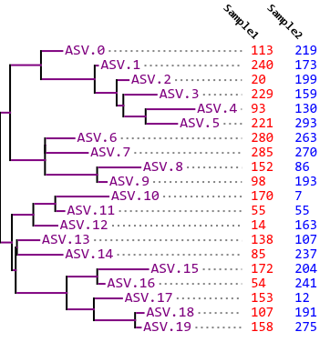
Fig. 10.1 Phylogram and feature table indicating which features (amplicon sequence variants or ASVs) are present in each of two samples. This example illustrates an Unweighted UniFrac distance of zero between the two samples.¶

In Fig. 10.1, all of the ASVs that are observed in either sample are observed in both samples. As a result, the unique branch length in this case is zero, so we have a UniFrac distance of 0 between Sample 1 and Sample 2.

$../_images/unifrac-tree-3.png$

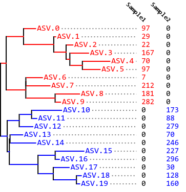
Fig. 10.2 Phylogram and feature table indicating which features (amplicon sequence variants or ASVs) are present in each of two samples. This example illustrates an Unweighted UniFrac distance of one between the two samples.¶

On the other end of the spectrum, in Fig. 10.2, all of the ASVs in the tree are observed either in Sample 1 or Sample 2, but not in both samples. Furthermore, the ASVs observed in each sample are segregated into different clades in the phylogenetic tree such that there is no overlapping branch length at all. The unique branch length is therefore equal to the observed branch length, so we have a UniFrac distance of 1 between Sample A and Sample B.

$../_images/unifrac-tree-2.png$

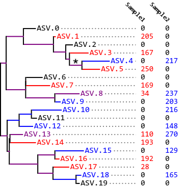
Fig. 10.3 Phylogram and feature table indicating which features (amplicon sequence variants or ASVs) are present in each of two samples. This example illustrates an Unweighted UniFrac distance of approximately 0.5 between the two samples. The * indicates a branch length that is observed in both samples because descendant ASVs are observed in both samples.¶

In most cases, our samples are somewhere between these extremes, as represented in Fig. 10.3. In this tree, some of our branch length is unique, and some is not. For example, ASV.5 is only observed in Sample 1, so the terminal branch leading to ASV.5 is red. ASV.4 is only observed in Sample 2, so the terminal branch leading to ASV.4 is blue. However, the last internal branch that leads to both ASV.5 and ASV.4 (annotated with *) is observed in both samples because ASVs in that lineage (ASV.5 and ASV.4) are observed in both samples. That branch is therefore colored purple. In this case, we have an intermediate UniFrac distance between Sample 1 and Sample 2, perhaps somewhere around 0.5.

10.1.3.2. Worked example of Unweighted UniFrac¶

Now let’s compute Unweighted UniFrac on our example feature table. We’ll work with the same phylogenetic tree that we used when computing Faith’s Phylogenetic Diversity. I’ll work through computing Unweighted UniFrac between samples 4ac2 and e375. Follow along with this computation, and then try computing Unweighted UniFrac distances between 4ac2 and 4gd8, and then between e375 and 4gd8. I’ll present the full distance matrix at the end of this section so you check your answers.

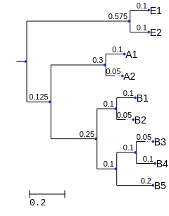
Fig. 10.4 A phylogenetic tree representing all of the features in our original feature table. (This tree isn’t intended to accurately represent the relationship between the Bacteria, Archaea, and Eukarya.)¶

Here’s the feature table again for convenience:

rarefied_feature_table_1.style

	B1	B2	B3	B4	A1	E2
4ac2	3	5	2	0	0	0
e375	3	4	1	2	0	0
4gd8	4	0	0	0	3	3

from io import StringIO
from skbio.tree import TreeNode

tree_1n = StringIO('((B1:0.1,B2:0.05):0.1,((B3:0.05,B4:0.1):0.1,B5:0.2):0.1,'
                   '((A1:0.1,A2:0.05):0.3,'
                   '(E1:0.1,E2:0.1):0.7):0.25);')

tree_1 = TreeNode.read(tree_1n)
tree_1 = tree_1.root_at_midpoint()

tree_1a = qiime2.Artifact.import_data("Phylogeny[Rooted]", tree_1)

To compute Unweighted UniFrac by hand, I recommend taking a similar approach to the one that you used for computing Faith’s Phylogenetic Diversity by hand. Print the phylogenetic tree Fig. 10.4, and get two colored pens. This time, for each of the two features, trace the branches from the observed tips to the root of the tree in a different color for each sample. As a reminder, if you sum those branch lengths of each color, each sum will be the Faith’s Phylogenetic Diversity for the corresponding sample.

def get_observed_nodes(tree, table, sample_id, verbose=False):
    if verbose:
        print("Observed branch lengths for sample %s" % sample_id)
        
    sample_vector = table.T[sample_id]
    observed_features = sample_vector.index[sample_vector.to_numpy().nonzero()[0]]
    observed_nodes = set()
    
    # iterate over the observed features
    for feature_id in observed_features:
        t = tree.find(feature_id)
        observed_nodes.add(t)
        if verbose:
            print(t.name, t.length, end=' ')
        for internal_node in t.ancestors():
            if internal_node.length is None:
                # we've hit the root
                if verbose: print('')
            else:
                if verbose and internal_node not in observed_nodes:
                    print(internal_node.length, end=' ')
                observed_nodes.add(internal_node)
    faith_pd = sum(o.length for o in observed_nodes)
    
    if verbose:
      print("Faith's Phylogenetic Diversity of sample %s: %1.2f" % (sample_id, faith_pd))
    return observed_nodes

sample_id1 = '4ac2'
sample_id2 = 'e375'

observed_nodes1 = get_observed_nodes(tree_1, rarefied_feature_table_1, sample_id1, verbose=True)
print('')
observed_nodes2 = get_observed_nodes(tree_1, rarefied_feature_table_1, sample_id2, verbose=True)

Observed branch lengths for sample 4ac2
B1 0.1 0.1 0.25 0.125 
B2 0.05 
B3 0.05 0.1 0.1 
Faith's Phylogenetic Diversity of sample 4ac2: 0.88

Observed branch lengths for sample e375
B1 0.1 0.1 0.25 0.125 
B2 0.05 
B3 0.05 0.1 0.1 
B4 0.1 
Faith's Phylogenetic Diversity of sample e375: 0.97

To compute Unweighted UniFrac, you’ll distinguish between branches that are traced in different ways. First, all of the branches that are colored (in either or both of your colors) are your Observed Branches. In the phylograms above (e.g., Fig. 10.3), the purple, blue, and red branches are the observed branches. The lengths of the observed branches are summed to give your Observed branch length. Each branch length should be included in the sum only one time.

observed_branches = observed_nodes1 | observed_nodes2
observed_branch_lengths = [o.length for o in observed_branches]
observed_branch_length = sum(observed_branch_lengths)    

print('Observed branch lengths = %s' % str(observed_branch_lengths))
print('Sum of observed branch lengths: %1.2f' % observed_branch_length)

Observed branch lengths = [0.25, 0.125, 0.05, 0.1, 0.1, 0.1, 0.1, 0.05, 0.1]
Sum of observed branch lengths: 0.97

Next, the branches that are colored in only one of the two colors are your Unique Branches. In the phylograms above (e.g., Fig. 10.3), the blue and red branches are the unique branches. The lengths of the unique branches are summed to give your Unique branch length.

shared_branches = observed_nodes1 & observed_nodes2
unique_branches = observed_branches - shared_branches
unique_branch_lengths = [u.length for u in unique_branches]
unique_branch_length = sum(unique_branch_lengths)

print('Unique branch lengths = %s' % str(unique_branch_lengths))
print('Sum of unique branch lengths: %1.2f' % unique_branch_length)

Unique branch lengths = [0.1]
Sum of unique branch lengths: 0.10

Dividing the unique branch length by the observed branch length tells you what fraction of the total observed branch length is unique to one of the samples. The more of the branch length that is unique to one of the samples, the more different the samples are from one another. This value is the Unweighted UniFrac distance (10.4) between the pair of samples.

unweighted_unifrac = unique_branch_length / observed_branch_length

print('Unweighted UniFrac = Unique branch length / Observed branch length')
print('Unweighted UniFrac = %1.2f / %1.2f' % (unique_branch_length, observed_branch_length))
print('Unweighted UniFrac between samples %s and %s = %1.2f' % 
            (sample_id1, sample_id2, unweighted_unifrac))

Unweighted UniFrac = Unique branch length / Observed branch length
Unweighted UniFrac = 0.10 / 0.97
Unweighted UniFrac between samples 4ac2 and e375 = 0.10

Computing Unweighted UniFrac between all pairs of the samples in the feature table results in the following distance matrix:

unweighted_unifrac_1a = div.actions.beta_phylogenetic(
                                         rarefied_feature_table_1a, 
                                         tree_1a, 
                                         metric='unweighted_unifrac').distance_matrix
unweighted_unifrac_1 = unweighted_unifrac_1a.view(skbio.DistanceMatrix).to_data_frame()
unweighted_unifrac_1.style.set_precision(2)

	4ac2	e375	4gd8
4ac2	0.00	0.10	0.71
e375	0.10	0.00	0.72
4gd8	0.71	0.72	0.00

10.1.4. Weighted UniFrac distance¶

10.2. Interpreting distance matrices¶

In the previous section we computed distance matrices that contained the pairwise distances between a few samples. You can look at those distance matrices and get a pretty good feeling for what the patterns are. For example, what are the most similar samples? What are the most dissimilar samples?

What if instead of three samples though, we had more. Here’s a screenshot from a distance matrix containing data on 105 samples (this is just the first few rows and columns):

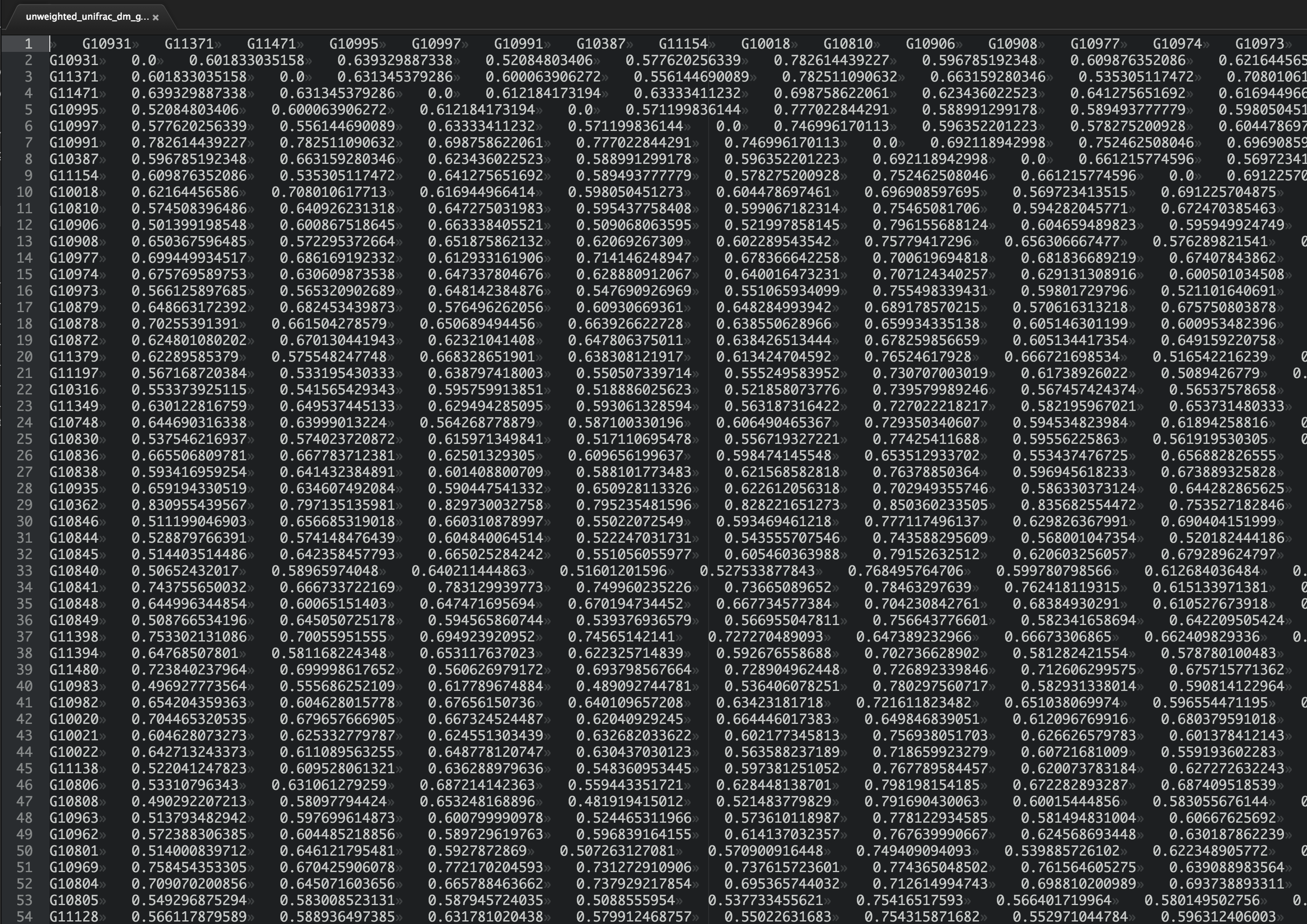
Do you have a good feeling for the patterns here? What are the most similar samples? What are the most dissimilar samples?

Chances are, you can’t just squint at that table and understand what’s going on (but if you can, I’m hiring!). The problem is exacerbated by the fact that in modern microbial ecology studies we may have thousands or tens of thousands of samples, not “just” hundreds as in the table above. We need tools to help us take these raw distances and convert them into something that we can interpret. In this section we’ll look at some techniques, one of which we’ve covered previously, that will help us interpret large distance matrices.

One excellent paper that includes a comparison of several different strategies for interpreting beta diversity results is Costello et al. Science (2009) Bacterial Community Variation in Human Body Habitats Across Space and Time. In this study, the authors collected microbiome samples from 7 human subjects at about 25 sites on their bodies, at four different points in time.

Figure 1 shows several different approaches for comparing the resulting UniFrac distance matrix (this image is linked from the Science journal website - copyright belongs to Science):

Let’s generate a small distance matrix representing just a few of these body sites, and figure out how we’d generate and interpret each of these visualizations. The values in the distance matrix below are a subset of the unweighted UniFrac distance matrix representing two samples each from three body sites from the Costello et al. (2009) study.

>>> sample_ids = ['A', 'B', 'C', 'D', 'E', 'F']
>>> _columns = ['body site', 'individual']
>>> _md = [['gut', 'subject 1'],
...        ['gut', 'subject 2'],
...        ['tongue', 'subject 1'],
...        ['tongue', 'subject 2'],
...        ['skin', 'subject 1'],
...        ['skin', 'subject 2']]
...
>>> human_microbiome_sample_md = pd.DataFrame(_md, index=sample_ids, columns=_columns)
>>> human_microbiome_sample_md
  body site individual
A       gut  subject 1
B       gut  subject 2
C    tongue  subject 1
D    tongue  subject 2
E      skin  subject 1
F      skin  subject 2

>>> dm_data = np.array([[0.00, 0.35, 0.83, 0.83, 0.90, 0.90],
...                     [0.35, 0.00, 0.86, 0.85, 0.92, 0.91],
...                     [0.83, 0.86, 0.00, 0.25, 0.88, 0.87],
...                     [0.83, 0.85, 0.25, 0.00, 0.88, 0.88],
...                     [0.90, 0.92, 0.88, 0.88, 0.00, 0.50],
...                     [0.90, 0.91, 0.87, 0.88, 0.50, 0.00]])
...
>>> human_microbiome_dm = DistanceMatrix(dm_data, sample_ids)
>>> print(human_microbiome_dm)
6x6 distance matrix
IDs:
'A', 'B', 'C', 'D', 'E', 'F'
Data:
[[ 0.    0.35  0.83  0.83  0.9   0.9 ]
 [ 0.35  0.    0.86  0.85  0.92  0.91]
 [ 0.83  0.86  0.    0.25  0.88  0.87]
 [ 0.83  0.85  0.25  0.    0.88  0.88]
 [ 0.9   0.92  0.88  0.88  0.    0.5 ]
 [ 0.9   0.91  0.87  0.88  0.5   0.  ]]

10.2.1. Distribution plots and comparisons¶

First, let’s look at the analysis presented in panels E and F. Instead of generating bar plots here, we’ll generate box plots as these are more informative (i.e., they provide a more detailed summary of the distribution being investigated). One important thing to notice here is the central role that the sample metadata plays in the visualization. If we just had our sample ids (i.e., letters A through F) we wouldn’t be able to group distances into within and between sample type categories, and we therefore couldn’t perform the comparisons we’re interested in.

>>> def within_between_category_distributions(dm, md, md_category):
...     within_category_distances = []
...     between_category_distances = []
...     for i, sample_id1 in enumerate(dm.ids):
...         sample_md1 = md[md_category][sample_id1]
...         for sample_id2 in dm.ids[:i]:
...             sample_md2 = md[md_category][sample_id2]
...             if sample_md1 == sample_md2:
...                 within_category_distances.append(dm[sample_id1, sample_id2])
...             else:
...                 between_category_distances.append(dm[sample_id1, sample_id2])
...     return within_category_distances, between_category_distances

>>> within_category_distances, between_category_distances = within_between_category_distributions(human_microbiome_dm, human_microbiome_sample_md, "body site")
>>> print(within_category_distances)
>>> print(between_category_distances)
[0.34999999999999998, 0.25, 0.5]
[0.82999999999999996, 0.85999999999999999, 0.82999999999999996, 0.84999999999999998, 0.90000000000000002, 0.92000000000000004, 0.88, 0.88, 0.90000000000000002, 0.91000000000000003, 0.87, 0.88]

>>> import seaborn as sns
>>> ax = sns.boxplot(data=[within_category_distances, between_category_distances])
>>> ax.set_xticklabels(['same body habitat', 'different body habitat'])
>>> ax.set_ylabel('Unweighted UniFrac Distance')
>>> _ = ax.set_ylim(0.0, 1.0)
<Figure size 432x288 with 1 Axes>

>>> from skbio.stats.distance import anosim
>>> anosim(human_microbiome_dm, human_microbiome_sample_md, 'body site')
method name               ANOSIM
test statistic name            R
sample size                    6
number of groups               3
test statistic                 1
p-value                    0.065
number of permutations       999
Name: ANOSIM results, dtype: object

If we run through these same steps, but base our analysis on a different metadata category where we don’t expect to see any significant clustering, you can see that we no longer get a significant result.

>>> within_category_distances, between_category_distances = within_between_category_distributions(human_microbiome_dm, human_microbiome_sample_md, "individual")
>>> print(within_category_distances)
>>> print(between_category_distances)
[0.82999999999999996, 0.84999999999999998, 0.90000000000000002, 0.88, 0.91000000000000003, 0.88]
[0.34999999999999998, 0.85999999999999999, 0.82999999999999996, 0.25, 0.92000000000000004, 0.88, 0.90000000000000002, 0.87, 0.5]

>>> ax = sns.boxplot(data=[within_category_distances, between_category_distances])
>>> ax.set_xticklabels(['same person', 'different person'])
>>> ax.set_ylabel('Unweighted UniFrac Distance')
>>> _ = ax.set_ylim(0.0, 1.0)
<Figure size 432x288 with 1 Axes>

>>> anosim(human_microbiome_dm, human_microbiome_sample_md, 'individual')
method name                 ANOSIM
test statistic name              R
sample size                      6
number of groups                 2
test statistic           -0.333333
p-value                      0.869
number of permutations         999
Name: ANOSIM results, dtype: object

Why do you think the distribution of distances between people has a greater range than the distribution of distances within people in this particular example?

Here we used ANOSIM testing whether our with and between category groups differ. This test is specifically designed for distance matrices, and it accounts for the fact that the values are not independent of one another. For example, if one of our samples was very different from all of the others, all of the distances associated with that sample would be large. It’s very important to choose the appropriate statistical test to use. One free resource for helping you do that is The Guide to Statistical Analysis in Microbial Ecology (GUSTAME). If you’re getting started in microbial ecology, I recommend spending some time studying GUSTAME.

10.2.2. Hierarchical clustering¶

Next, let’s look at a hierarchical clustering analysis, similar to that presented in panel G above. Here I’m applying the UPGMA functionality implemented in SciPy to generate a tree which we visualize with a dendrogram. However the tips in this tree don’t represent sequences or OTUs, but instead they represent samples, and samples with a smaller branch length between them are more similar in composition than samples with a longer branch length between them. (Remember that only horizontal branch length is counted - vertical branch length is just to aid in the organization of the dendrogram.)

>>> from scipy.cluster.hierarchy import average, dendrogram
>>> lm = average(human_microbiome_dm.condensed_form())
>>> d = dendrogram(lm, labels=human_microbiome_dm.ids, orientation='right',
...                link_color_func=lambda x: 'black')
<Figure size 432x288 with 1 Axes>

Again, we can see how the data really only becomes interpretable in the context of metadata:

>>> labels = [human_microbiome_sample_md['body site'][sid] for sid in sample_ids]
>>> d = dendrogram(lm, labels=labels, orientation='right',
...                link_color_func=lambda x: 'black')
<Figure size 432x288 with 1 Axes>

>>> labels = [human_microbiome_sample_md['individual'][sid] for sid in sample_ids]
>>> d = dendrogram(lm, labels=labels, orientation='right',
...                link_color_func=lambda x: 'black')
<Figure size 432x288 with 1 Axes>

10.2.3. Ordination¶

Finally, let’s look at ordination, similar to that presented in panels A-D. The basic idea behind ordination is dimensionality reduction: we want to take high-dimensionality data (a distance matrix) and represent that in a few (usually two or three) dimensions. As humans, we’re very bad at interpreting high dimensionality data directly: with ordination, we can take an $n$-dimensional data set (e.g., a distance matrix of shape $n \times n$, representing the distances between $n$ biological samples) and reduce that to a 2-dimensional scatter plot similar to that presented in panels A-D above.

Ordination is a technique that is widely applied in ecology and in bioinformatics, but the math behind some of the methods such as Principal Coordinates Analysis is fairly complex, and as a result I’ve found that these methods are a black box for a lot of people. Possibly the most simple ordination technique is one called Polar Ordination. Polar Ordination is not widely applied because it has some inconvenient features, but I find that it is useful for introducing the idea behind ordination. Here we’ll work through a simple implementation of ordination to illustrate the process, which will help us to interpret ordination plots. In practice, you will use existing software, such as scikit-bio’s ordination module.

An excellent site for learning more about ordination is Michael W. Palmer’s Ordination Methods page.

10.3. List of works cited¶

LK05: Catherine Lozupone and Rob Knight. UniFrac: a new phylogenetic method for comparing microbial communities. Appl. Environ. Microbiol., 71(12):8228–8235, December 2005.

q2book

Beta diversity

Contents